nigel delaney

First Blog Post: Not All Poisson Random Variables Are Created Equally

Thursday, September 20, 2012

Update: Post moved to a new place that allows for comments

Spurred by a slow running program, I spent an afternoon researching what algorithms are available for generating Poisson random variables and figuring out which methods are used by R, Matlab, NumPy, the GNU Science Libraray and various other available packages. I learned some things that I think would be useful to have on the internet somewhere, so I thought it would be good material for a first blog post.

Many meaningfully different algorithms exists to simulate from a Poisson distribution and commonly used code libraries and programs have not settled on the same method. I found some of the available tools use inefficient methods, though figuring out which method a package used often required me to  work through the source code.

This blog post explains the specific algorithms that commonly used packages implement. For those looking for the quick take away, the lesson is to avoid the default Matlab implementation and the GNU Science Library (GSL).

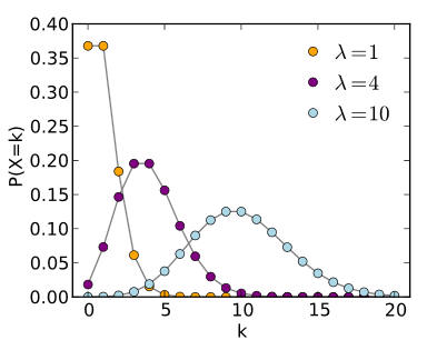
For context, when deciding which Poisson simulation routine to use there are essentially two important questions. The first is if you will be repeatedly simulating values conditioned on the same mean parameter value (λ).  If so, methods that that store certain pre-computed information offer very big performance improvements.  However, essentially no package implements these routines (with some exceptions discussed at the end).  The second question is if you are frequently going to simulate with a λ > 10.  Poisson simulation methods usually switch between two different methods depending on if λ is above or below 10 (this "decision value" can change slightly but seems to always be >=10).  When λ is below 10, the algorithms are all very similar and their speed scales with the value of λ.  Where the algorithms really differ is how fast they are when  λ > 10.

For λ > 10, the GNU Science Library (GSL) and Matlab have slower algorithms that are of order log(λ).  Their methods are straightforward implementations from pages 137-138 of Knuth's Seminumerical Algorithms book  (specifically the 1998 version, older versions had a more inaccurate algorithm). On these pages Knuth's book presents a 1974 algorithm by Aherns and Dieter [1] but he unfortunately only introduces the more efficient algorithm from Aherns and Dieters' 1982 paper [2] with an excercise buried at the end of the chapter.  This was an understandable decision given the complexity of the 1982 method, but it is somewhat unfortunate for Matlab and GSL users.

A major breakthrough in algorithms for Poisson random generators came with the publication of the first O(1) algorithm in 1979 by Atkinson [3] and methods from then on are signifcantly better. The Math.NET project uses this 1979 algorithm in their sampler.  A still better method is the 1982 Aherns and Dieter method which is also heavily used.  For example, the R Project uses this efficient algorithm.  Importantly, the R version also checks to see if it can avoid recomputing values if the same λ value is being used on repeated function calls. To me, this is just another example of how great the core R implementations often are.  Although in my field the GSL seems to dominate when people code, I think a reason for this is that a lot of people don't realize that many R functions can be easily incorporated into C/C++ code using the R Stand Alone Math Library.  I have found simulating with the R libraries has many advantages over using the GSL. 

In 1986 Luc Devroye published a real tome on Random Variate Generation (that is freely available online).  Within it was a very good algorithm, which I gather is based on a 1981 paper, that is currently implemented by the Infer .NET package and the Apache Commons Math Java library.  The algorithm is given on page 511 of the book, but anyone independently implementing it should be aware that the published errata corrects some errors in the original publication of this algorithm (Infer.NET has these corrections, but I didn't check for them in the Apache Commons library).

The most modern algorithm I found implemented was a 1993 algorithm by Hormann [5], which his benchmarks showed either outperformed other algorithms at many λ values, or was not that meaningfully slower over a narrower range of λ values. Numpy implements this routine, and it seems at least one commentator on another blog implemented it as well.

So which to use?  I think one should make sure they are using a post-1979 algorithm (so not Matlab or GSL).  Routines after this point are similar enough that if simulating Poisson variables is still the bottleneck one should benchmark available code that implements these different options.  At this point the coding/implementation specifics, and the ease of using that library, will likely be more important than the algorithm.  If no available option adequately performs, the algorithms in [2], [4] and [5] can be evaluated for application to a specific usage scenario, though by then it is probably worth knowing that the algorithms that are truly the fastest have efficient pre-computed tables or a particular λ  value [6] .  One such table lookup method from reference [6] is implemented in Matlab code available from an open source file exchange here.  Though I did not completely evaluate [6], the 2004 paper says it can outperform (5X-15X faster) the other algorithms I have discussed.  However, after a quick run through of the paper, I couldn't tell if the benchmarks in [6] were based on repeated simulations from the same λ value, or with constantly changing λ values (I suspect it is the former which is why this algorithm is not widely adopted).  The algorithm in [6] strikes me as very efficient for the same λ value, and C code for it is available from the publishing journal.  Interestingly, a Matlab benchmark test shows this method is about 10X faster than the default poissrnd Matlab function, even though it recreates the required look up tables on each function call.  However, I suspect the performance increase is slightly exaggerated because the original Matlab function has such a slow routine and this method switches directly to the normal approximation of the Poisson distribution when λ is over 1,000.  This shortcut could easily be incorporated to every other method mentioned, though the direct methods seem fast enough that I personally would not like to muck around evaluating how well one distribution mathematically approximates another distribution that itself is only approximating a complex reality.

Which brings me to the end of the first blog post.  If you are still reading this you slogged through some insights gained from someone who just read Fortran code and academic papers from a time when Nirvana was still just a Buddhist goal and not a grunge rock band.  Hopefully it prevents someone else from doing the same.

References

1. Ahrens JH, Dieter U (1974) Computer methods for sampling from gamma, beta, poisson and bionomial distributions. Computing 12: 223-246.
2. Ahrens JH, Dieter U (1982) Computer generation of Poisson deviates from modified normal distributions. ACM Transactions on Mathematical Software (TOMS) 8: 163-179.
3. Atkinson A (1979) The computer generation of Poisson random variables. Applied Statistics: 29-35.
4. Devroye L (1986) Non-uniform random variate generation: Springer-Verlag New York.
5. Hörmann W (1993) The transformed rejection method for generating Poisson random variables. Insurance: Mathematics and Economics 12: 39-45.
6. Marsaglia G, Tsang WW, Wang J (2004) Fast generation of discrete random variables. Journal of Statistical Software 11: 1-11.